Interquartile range: Difference between revisions
m unbalanced curley brackets |
Fixed version. Tags: Reverted possible vandalism references removed Visual edit |
||
| Line 1: | Line 1: | ||
{{Short description|Measure of statistical dispersion}} |
{{Short description|Measure of statistical dispersion}} |
||
{{Redirect|IQR}} |
{{Redirect|IQR}}[[Interquartile range]] |
||
| ⚫ | |||
# '''Definition''': |
|||
In [[descriptive statistics]], the '''interquartile range''' ('''IQR''') is a measure of [[statistical dispersion]], which is the spread of the data.<ref name=":1">{{Cite book|last=Dekking|first=Frederik Michel|url=http://link.springer.com/10.1007/1-84628-168-7|title=A Modern Introduction to Probability and Statistics|last2=Kraaikamp|first2=Cornelis|last3=Lopuhaä|first3=Hen Paul|last4=Meester|first4=Ludolf Erwin|date=2005|publisher=Springer London|isbn=978-1-85233-896-1|series=Springer Texts in Statistics|location=London|doi=10.1007/1-84628-168-7}}</ref> The IQR may also be called the '''midspread''', '''middle 50%''', '''fourth spread''', or '''H‑spread.''' It is defined as the difference between the 75th and 25th [[percentiles]] of the data.<ref name="Upton" /><ref name="ZK" /><ref>{{Cite book|last=Ross|first=Sheldon|title=Introductory Statistics|publisher=Elsevier|year=2010|isbn=978-0-12-374388-6|location=Burlington, MA|pages=103–104}}</ref> To calculate the IQR, the data set is divided into [[quartile]]s, or four rank-ordered even parts via linear interpolation.<ref name=":1" /> These quartiles are denoted by Q<sub>1</sub> (also called the lower quartile), ''Q''<sub>2</sub> (the [[median]]), and ''Q''<sub>3</sub> (also called the upper quartile). The lower quartile corresponds with the 25th percentile and the upper quartile corresponds with the 75th percentile, so IQR = ''Q''<sub>3</sub> − ''Q''<sub>1</sub><ref name=":1" /><sub>.</sub> |
|||
#* The '''IQR''' is a measure of statistical dispersion, representing the '''spread''' of data. |
|||
#* It is the difference between the '''75th percentile (Q3)''' and the '''25th percentile (Q1)''' of a dataset. |
|||
#* [[Interquartile range|Also known as the '''midspread''', '''middle 50%''', or '''H-spread''' <sup>1</sup>]]. |
|||
# '''Calculation''': |
|||
#* To find the IQR: |
|||
#** Subtract the '''Q1''' value from the '''Q3''' value: |
|||
#*** '''IQR = Q3 - Q1''' |
|||
#** '''Q1''' is the value below which '''25%''' of the data lies. |
|||
#** '''Q3''' is the value below which '''75%''' of the data lies. |
|||
#** Think of '''Q1''' as the median of the first half and '''Q3''' as the median of the second half of the distribution <sup>2</sup>. |
|||
# '''Methods for Finding Quartiles''': |
|||
#* There are two commonly used methods: |
|||
#** '''Exclusive Method''': Excludes the median when identifying '''Q1''' and '''Q3'''. |
|||
#** '''Inclusive Method''': Includes the median in identifying the quartiles. |
|||
#* The choice depends on whether the dataset has an odd or even number of data points <sup>2</sup>. |
|||
# '''Usefulness''': |
|||
#* The IQR assesses variability where most of the values lie. |
|||
#* Larger IQR values indicate that the central portion of the data spreads out further <sup>3</sup>. |
|||
| ⚫ | |||
| ⚫ | The IQR is an example of a [[trimmed estimator]], defined as the 25% trimmed [[Range (statistics)|range]], which enhances the accuracy of dataset statistics by dropping lower contribution, outlying points.<ref name=":2">{{Cite book|last=Kaltenbach|first=Hans-Michael|url=https://www.worldcat.org/oclc/763157853|title=A concise guide to statistics|date=2012|publisher=Springer|isbn=978-3-642-23502-3|location=Heidelberg|oclc=763157853}}</ref> It is also used as a [[Robust measures of scale|robust measure of scale]]<ref name=":2" /> It can be clearly visualized by the box on a [[box plot]].<ref name=":1" /> |
||
| ⚫ | The IQR is an example of a [[trimmed estimator]], defined as the 25% trimmed [[Range (statistics)|range]], which enhances the accuracy of dataset statistics by dropping lower contribution, outlying points.<ref name=":2">{{Cite book|last=Kaltenbach|first=Hans-Michael|url=https://www.worldcat.org/oclc/763157853|title=A concise guide to statistics|date=2012|publisher=Springer|isbn=978-3-642-23502-3|location=Heidelberg|oclc=763157853}}</ref> It is also used as a [[Robust measures of scale|robust measure of scale]]<ref name=":2" /> It can be clearly visualized by the box on a [[box plot]].<ref name=":1">{{Cite book |last=Dekking |first=Frederik Michel |url=http://link.springer.com/10.1007/1-84628-168-7 |title=A Modern Introduction to Probability and Statistics |last2=Kraaikamp |first2=Cornelis |last3=Lopuhaä |first3=Hen Paul |last4=Meester |first4=Ludolf Erwin |date=2005 |publisher=Springer London |isbn=978-1-85233-896-1 |series=Springer Texts in Statistics |location=London |doi=10.1007/1-84628-168-7}}</ref> |
||
==Use== |
==Use== |
||
Revision as of 04:50, 19 April 2024
- Definition:
- The IQR is a measure of statistical dispersion, representing the spread of data.
- It is the difference between the 75th percentile (Q3) and the 25th percentile (Q1) of a dataset.
- Also known as the midspread, middle 50%, or H-spread 1.
- Calculation:
- To find the IQR:
- Subtract the Q1 value from the Q3 value:
- IQR = Q3 - Q1
- Q1 is the value below which 25% of the data lies.
- Q3 is the value below which 75% of the data lies.
- Think of Q1 as the median of the first half and Q3 as the median of the second half of the distribution 2.
- Subtract the Q1 value from the Q3 value:
- To find the IQR:
- Methods for Finding Quartiles:
- There are two commonly used methods:
- Exclusive Method: Excludes the median when identifying Q1 and Q3.
- Inclusive Method: Includes the median in identifying the quartiles.
- The choice depends on whether the dataset has an odd or even number of data points 2.
- There are two commonly used methods:
- Usefulness:
- The IQR assesses variability where most of the values lie.
- Larger IQR values indicate that the central portion of the data spreads out further 3.
Remember, the IQR provides valuable insights into the spread of data, especially within the middle 50% of your dataset.

The IQR is an example of a trimmed estimator, defined as the 25% trimmed range, which enhances the accuracy of dataset statistics by dropping lower contribution, outlying points.[1] It is also used as a robust measure of scale[1] It can be clearly visualized by the box on a box plot.[2]
Use
Unlike total range, the interquartile range has a breakdown point of 25%[3] and is thus often preferred to the total range.
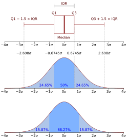
The IQR is used to build box plots, simple graphical representations of a probability distribution.
The IQR is used in businesses as a marker for their income rates.
For a symmetric distribution (where the median equals the midhinge, the average of the first and third quartiles), half the IQR equals the median absolute deviation (MAD).
The median is the corresponding measure of central tendency.
The IQR can be used to identify outliers (see below). The IQR also may indicate the skewness of the dataset.[2]
The quartile deviation or semi-interquartile range is defined as half the IQR.[4]
Algorithm
The IQR of a set of values is calculated as the difference between the upper and lower quartiles, Q3 and Q1. Each quartile is a median[5] calculated as follows.
Given an even 2n or odd 2n+1 number of values
- first quartile Q1 = median of the n smallest values
- third quartile Q3 = median of the n largest values[5]
The second quartile Q2 is the same as the ordinary median.[5]
Examples
Data set in a table
The following table has 13 rows, and follows the rules for the odd number of entries.
| i | x[i] | Median | Quartile |
|---|---|---|---|
| 1 | 7 | Q2=87 (median of whole table) |
Q1=31 (median of lower half, from row 1 to 6) |
| 2 | 7 | ||
| 3 | 31 | ||
| 4 | 31 | ||
| 5 | 47 | ||
| 6 | 75 | ||
| 7 | 87 | ||
| 8 | 115 | Q3=119 (median of upper half, from row 8 to 13) | |
| 9 | 116 | ||
| 10 | 119 | ||
| 11 | 119 | ||
| 12 | 155 | ||
| 13 | 177 |
For the data in this table the interquartile range is IQR = Q3 − Q1 = 119 - 31 = 88.
Data set in a plain-text box plot
                             +−−−−−+−+
               * |−−−−−−−−−−−|     | |−−−−−−−−−−−|
                             +−−−−−+−+

 +−−−+−−−+−−−+−−−+−−−+−−−+−−−+−−−+−−−+−−−+−−−+−−−+   number line
 0   1   2   3   4   5   6   7   8   9   10  11  12
For the data set in this box plot:
- Lower (first) quartile Q1 = 7
- Median (second quartile) Q2 = 8.5
- Upper (third) quartile Q3 = 9
- Interquartile range, IQR = Q3 - Q1 = 2
- Lower 1.5*IQR whisker = Q1 - 1.5 * IQR = 7 - 3 = 4. (If there is no data point at 4, then the lowest point greater than 4.)
- Upper 1.5*IQR whisker = Q3 + 1.5 * IQR = 9 + 3 = 12. (If there is no data point at 12, then the highest point less than 12.)
- Pattern of latter two bullet points: If there are no data points at the true quartiles, use data points slightly "inland" (closer to the median) from the actual quartiles.
This means the 1.5*IQR whiskers can be uneven in lengths. The median, minimum, maximum, and the first and third quartile constitute the Five-number summary.[6]
Distributions
The interquartile range of a continuous distribution can be calculated by integrating the probability density function (which yields the cumulative distribution function—any other means of calculating the CDF will also work). The lower quartile, Q1, is a number such that integral of the PDF from -∞ to Q1 equals 0.25, while the upper quartile, Q3, is such a number that the integral from -∞ to Q3 equals 0.75; in terms of the CDF, the quartiles can be defined as follows:
where CDF−1 is the quantile function.
The interquartile range and median of some common distributions are shown below
| Distribution | Median | IQR |
|---|---|---|
| Normal | μ | 2 Φ−1(0.75)σ ≈ 1.349σ ≈ (27/20)σ |
| Laplace | μ | 2b ln(2) ≈ 1.386b |
| Cauchy | μ | 2γ |
Interquartile range test for normality of distribution
The IQR, mean, and standard deviation of a population P can be used in a simple test of whether or not P is normally distributed, or Gaussian. If P is normally distributed, then the standard score of the first quartile, z1, is −0.67, and the standard score of the third quartile, z3, is +0.67. Given mean = and standard deviation = σ for P, if P is normally distributed, the first quartile
and the third quartile
If the actual values of the first or third quartiles differ substantially[clarification needed] from the calculated values, P is not normally distributed. However, a normal distribution can be trivially perturbed to maintain its Q1 and Q2 std. scores at 0.67 and −0.67 and not be normally distributed (so the above test would produce a false positive). A better test of normality, such as Q–Q plot would be indicated here.
Outliers

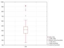
The interquartile range is often used to find outliers in data. Outliers here are defined as observations that fall below Q1 − 1.5 IQR or above Q3 + 1.5 IQR. In a boxplot, the highest and lowest occurring value within this limit are indicated by whiskers of the box (frequently with an additional bar at the end of the whisker) and any outliers as individual points.
See also
- Interdecile range – Statistical measure
- Midhinge – average of the first and third quartiles
- Probable error
- Robust measures of scale – Statistical indicators of the deviation of a sample
References
- ^ a b Kaltenbach, Hans-Michael (2012). A concise guide to statistics. Heidelberg: Springer. ISBN 978-3-642-23502-3. OCLC 763157853.
- ^ a b Dekking, Frederik Michel; Kraaikamp, Cornelis; Lopuhaä, Hen Paul; Meester, Ludolf Erwin (2005). A Modern Introduction to Probability and Statistics. Springer Texts in Statistics. London: Springer London. doi:10.1007/1-84628-168-7. ISBN 978-1-85233-896-1.
- ^ Rousseeuw, Peter J.; Croux, Christophe (1992). Y. Dodge (ed.). "Explicit Scale Estimators with High Breakdown Point" (PDF). L1-Statistical Analysis and Related Methods. Amsterdam: North-Holland. pp. 77–92.
- ^ Yule, G. Udny (1911). An Introduction to the Theory of Statistics. Charles Griffin and Company. pp. 147–148.
- ^ a b c Bertil., Westergren (1988). Beta [beta] mathematics handbook : concepts, theorems, methods, algorithms, formulas, graphs, tables. Studentlitteratur. p. 348. ISBN 9144250517. OCLC 18454776.
- ^ Dekking, Kraaikamp, Lopuhaä & Meester, pp. 235–237
Cite error: A list-defined reference named "Upton" is not used in the content (see the help page).
External links
 Media related to Interquartile range at Wikimedia Commons


